A friend recently asked me where the inductor equation comes from. Around the same time, I was looking into discrete nonlinear inductor models. To test different alternatives, I needed a continuous reference. Since it had been a while since I thought about coils and fields, I figured it was time to go back to basics.
Table of Contents
Open Table of Contents
1. The Relevant Maxwell Equations
Here are the equations we’ll need. The physics of inductors rests on two of Maxwell’s equations and one constitutive relation:
- (Ampère’s Law)
- (Faraday’s Law)
- (Constitutive Relation)
The idea is:
- Use Ampère to find from the current
- Use the constitutive relation to get
- Use Faraday to get the induced voltage
The result is the inductor equation
Two remarks. First, is really , the integral of current density over the surface. For discrete wires, this just means counting how many times the wire pierces the surface.
Second, the full Ampère’s Law includes a displacement current term:
For power inductors, the displacement current term is negligible: the device is tiny compared to the electromagnetic wavelength at typical operating frequencies, so the fields adjust almost instantaneously. In other words, we can drop the term entirely. This is called the quasi-static regime, and it lets us use the static form of Ampère’s Law at each instant.
2. The and Fields
The key to understanding power inductors is separating two concepts that often get tangled together: the magnetic field strength , which is the effort applied by the circuit, and the magnetic flux density , the response of the magnetic core.
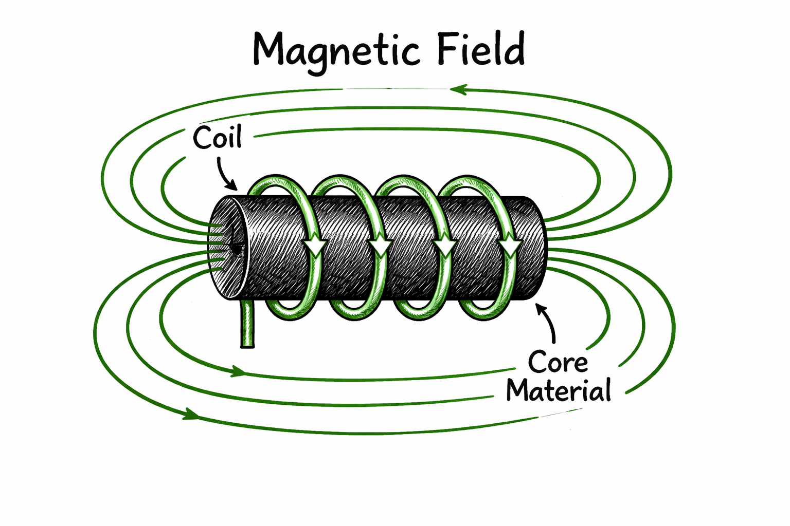
2.1 Magnetic Field Strength ()
The magnetic field strength is the driving force generated by the current flowing through the coil. It is defined rigorously by Ampère’s Law in integral form:
This states that the line integral of along a closed loop equals the total free current passing through the surface bounded by that loop.
Applying Ampère’s Law to a Solenoid
To find the field inside the coil, we define a rectangular Amperian loop of length that cuts through the windings.
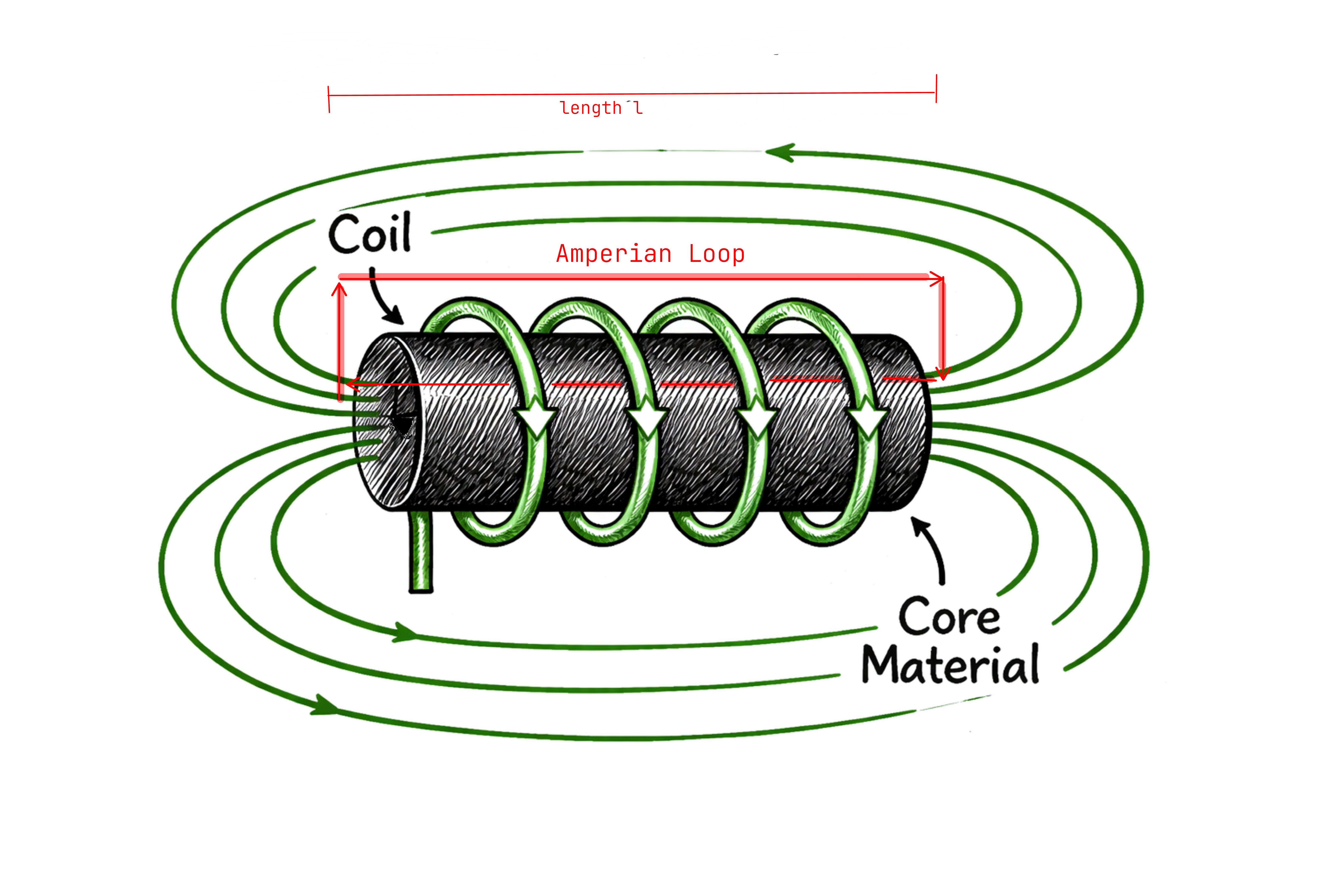
Inside the core, is parallel to the path (by the right-hand rule). Outside, it is negligible. Assuming the field is uniform within the core, the line integral simplifies to
If the loop encloses turns of wire, each carrying current , the enclosed current is
and therefore
Notice that is purely geometric: it depends only on the current and the winding density , not on the core material.
Why is the field negligible outside?
This commonly stated assumption deserves justification, but I couldn’t find a simple one beyond “experience says so”. One can use the Biot-Savart law to compute the external field and get estimates, but I chose to trust established wisdom and moved on.
Griffiths offers reasonable intuition: for an infinitely long solenoid, the external field is exactly zero. For a finite solenoid, it’s not strictly zero, but becomes negligible when the length is large compared to the diameter. The idea is that field lines close through the core, and the return path outside spreads over such a large volume that the field strength becomes tiny. In power inductors, the high-permeability core concentrates the flux even more, making the external field negligible for practical purposes.
Free vs. Bound Currents
I said above that is independent of the core material. This is because Ampère’s Law uses free current, which must be distinguished from microscopic currents inside the core:
- Free Current: The macroscopic current flowing through the wire (what we measure with an ammeter).
- Bound Current: Microscopic currents from electrons orbiting atoms and spinning on their axes inside the core. These create the material’s magnetization but are bound to their atoms.
Maxwell’s equations define to depend only on free current, so we can compute from the wire current alone. The core material shows up when we relate to .
2.2 Magnetic Flux Density ()
So is the “effort applied by the current”. The flux density is what the material gives back: the actual magnetic field inside the core. The two are related by the constitutive relation:
Remark on field lines. You’ll often hear described as “density of magnetic field lines.” The idea: pick a few starting points and trace curves that follow the field direction. Where lines bunch together, the field is strong. Where they spread apart, it’s weak. This only works as a comparison between regions (in a uniform field, the lines are parallel and equally spaced, so there’s no “bunching” to see). Still, it’s why people say that evaluating the flux () amounts to “counting how many lines pass through a surface.” A useful intuition, but as Feynman warns in his lectures, the picture has limitations and shouldn’t be pushed too far.
Unlike , depends heavily on the material: a high-permeability material “magnifies” the field.
2.3 Permeability ()
Permeability measures how easily a material aligns its internal magnetic domains with the external field:
- (Permeability of Free Space): H/m.
- (Relative Permeability): Dimensionless.
- Air:
- Ferrite/Iron:
A core with generates a -field 2000 times stronger than an air core for the same current.
Physical Origin: Bound Currents
Relative permeability is the multiplier we care about. It says how much bound current the material recruits internally.
The total flux density inside the core decomposes into the externally driven part and the material’s contribution,
where is the magnetization (magnetic moment per unit volume). The engineering definition groups both effects into a single multiplier,
so that
Since magnetization is proportional to bound surface current and is proportional to free current, this is approximately
For example, if a ferrite core has , then and the material does 99.95% of the work in creating the flux.
2.4 Magnetic Flux ()
The average value of the normal component of the field through a surface times the area of that surface is the magnetic flux through that surface:
This integral appears on the right-hand side of Faraday’s Law. Introducing here is primarily for convenience. But defining it clarifies why is called the flux density: it is the physical field that must be integrated to obtain the flux, which is ultimately our quantity of interest.
In a solenoid, the right-hand rule tells us that points along the core axis. If we take a cross-sectional cut through the core, the field is perpendicular to that surface, so and the integral simplifies to
3. From Magnetic Flux to Inductance
3.1 The Physics of Terminal Voltage
Faraday’s Law applies to the circulation of an electric field around a closed loop, but an inductor is an open circuit with two terminals. To get from a closed-loop integral to a voltage across terminals, we apply Faraday’s Law to a specific loop that follows the coil wire from start to finish, and then loop back in the air gap (outside the inductor) to close the loop:
Inside the Wire (Path A): The wire is a conductor, so along path A. The integral vanishes.
Across the Gap (Path B): Since the wire contributes nothing to the integral, the entire Electromotive Force (EMF) must appear across the gap:
This line integral is exactly the definition of voltage between two terminals. Following standard circuit conventions (defining voltage to oppose current change), we drop the negative sign:
Why is this voltage unique?
Strictly speaking, in time-varying magnetic fields, voltage is path-dependent. However, in circuit theory, we work under the Lumped Element Approximation. We suppose that change in the magnetic flux is mostly contained inside the core. Accordingly, the electric field in the air gap is conservative (), and line integrals outside the inductor do not depend on the path. This ensures that the voltage measured across the terminals is well-defined and doesn’t depend on how you arrange your voltmeter leads. This is why in nodal analysis, it makes sense to work with nodal voltages (potential voltage at terminals).
In some applications this approximation breaks down: parts of the circuit couple through the field across the air gap.
3.2 Flux Linkage and Inductance
An inductor consists of a coil with turns in series (think of it as coils of a single turn one after the other). So breaking out the path integral of the previous section, we find that the total voltage is the sum of the voltages induced in each turn:
This leads to the concept of flux linkage, , which is the total effective flux with the contribution of all turns. By Faraday’s law, the inductor’s voltage is then the rate of change of flux linkage:
Now, we can find a formula for the inductance , based on datasheet parameters.
Combining the flux linkage , the flux through one turn , and the H-field from Ampère’s Law gives the relationship between flux linkage and current:
The constant of proportionality is the inductance, :
which satisfies
The Factor
- First (Ampère): turns create the magnetic field ().
- Second (Faraday): turns harvest the voltage ().
4. The Physics of Saturation
Saturation is the main limitation of magnetic cores. It happens when the magnetic domains are fully aligned and can’t contribute any more flux.
4.1 The Mechanism
The permeability represents the ability of microscopic magnetic domains to align with :
- Linear Region: Domains are available and is high (e.g., ).
- Saturation: All domains aligned. The material cannot contribute further and drops toward .
4.2 The B-H Curve
The relationship between (drive) and (response) is nonlinear:
- Linear Region: Small currents. Domains align easily. The slope () is steep and constant.
- Saturation Knee: Most domains aligned. More energy () yields diminishing returns in .
- Hard Saturation: All domains aligned. The material acts like air.
4.3 Consequences of Saturation
When a core saturates, drops from thousands to approximately 1:
- decreases dramatically.
- collapses (since ).
- In , if while is maintained, then .
The current spikes uncontrollably and can destroy power switches.
5. A Smooth Saturation Model
Let’s build a model that captures the smooth roll-off into saturation. Real ferrites don’t have a sharp knee. They bend gradually.
5.1 Model Structure
The model has two parts:
- The ferromagnetic core is modeled by the hyperbolic tangent () function, which provides the smooth saturation knee.
- The air contribution is a linear term that represents the residual inductance () when the core is fully saturated (acting like an air-core inductor). It’s typically a small fraction of the unsaturated inductance.
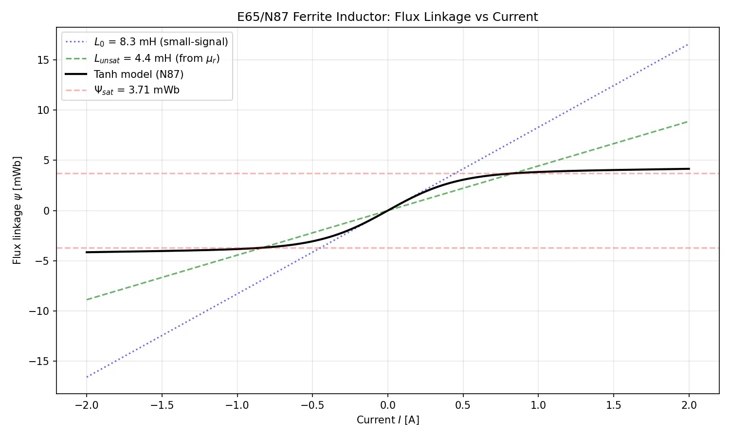
We model the flux linkage as a function of current using a hyperbolic tangent plus a linear term:
where:
- is the saturation flux linkage
- is the critical current
- is the unsaturated inductance
- is the residual inductance when fully saturated
- is the sharpness factor
and
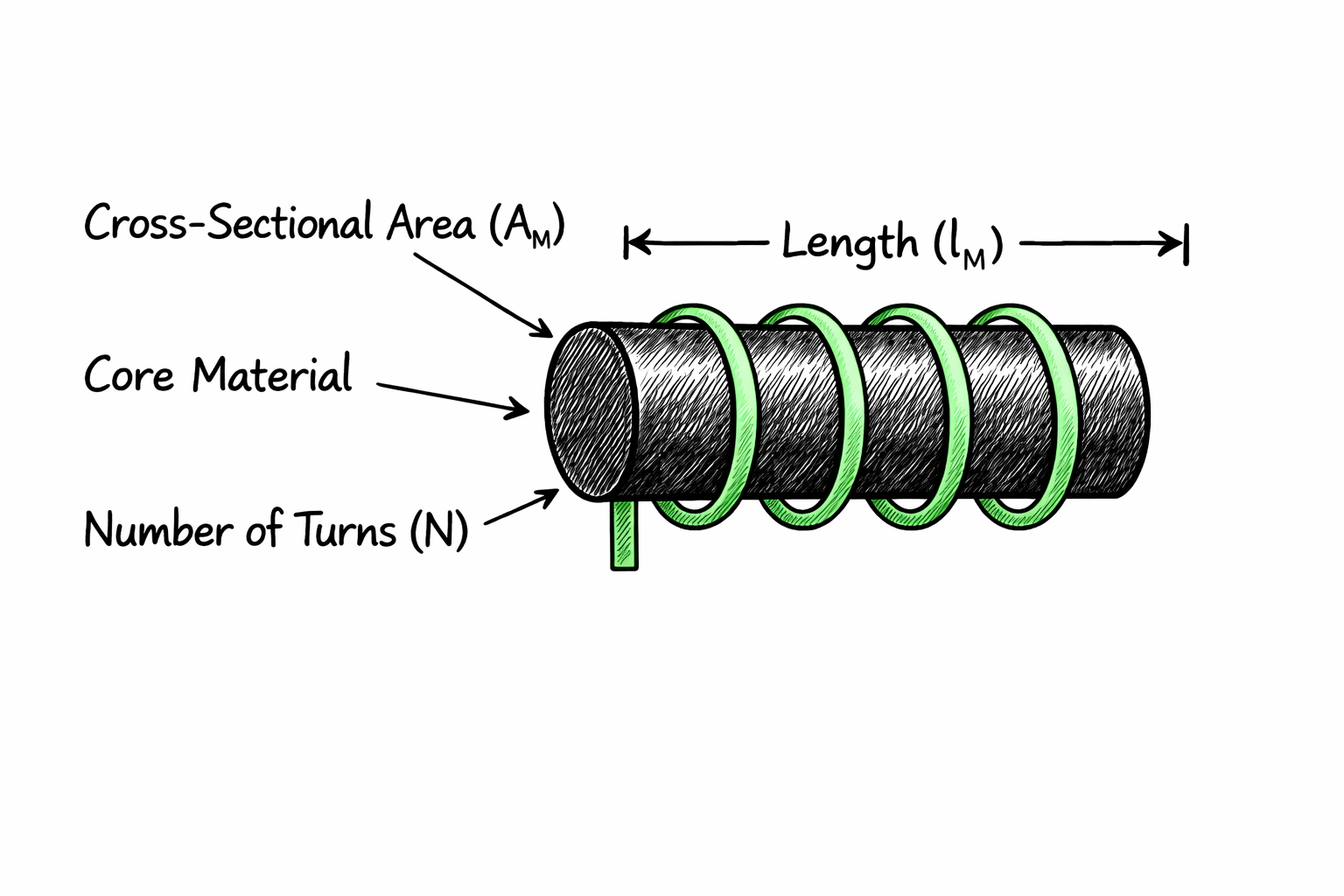
| Symbol | Description | Unit |
|---|---|---|
| Number of turns | - | |
| Cross-section area | m² | |
| Magnetic path length | m | |
| Permeability of free space | H/m | |
| Relative permeability | - |
5.2 The Sharpness Factor
The standard function has a fixed curvature that begins flattening relatively early. Real N87 ferrite maintains high permeability longer, then saturates more abruptly.
The sharpness factor compresses the x-axis:
- Steepens the initial slope (higher effective permeability)
- Causes saturation at lower current (moves the knee toward the -axis)
- Creates a quicker, more abrupt transition matching high-grade power ferrites
5.3 Linear Model for Small Signals
For the companion model validation, we need the small-signal inductance at :
Note that when . The sharpness factor effectively increases the apparent permeability for small signals.
6. Example: E65/N87 Power Inductor
A common combination in power electronics is the E65 core geometry with N87 ferrite material.
Note on core geometry: The derivations above assume a simple solenoid, but E65 is an E-core (shaped like the letter E). For such cores, manufacturers provide effective cross-sectional area and effective magnetic path length that account for the non-uniform geometry. These effective parameters allow the solenoid formulas to be applied directly. The values below are the effective parameters for an E65/32/27 core set.
Note on air gaps: The example below uses an ungapped core, resulting in a low critical current (0.84 A). In practice, power inductors almost always include an air gap, which reduces the effective permeability (e.g., from 2500 to 50–200) and proportionally increases the saturation current. The gap also stores most of the magnetic energy and linearizes the B-H curve, making inductance more stable over a wider current range.
| Designation | Category | Parameters |
|---|---|---|
| E65 | Core geometry | m², m |
| N87 | Core material | , T |
6.1 Computed Parameters
With turns:
| Parameter | Formula | Value |
|---|---|---|
| Base inductance | 4.44 mH | |
| Saturation flux linkage | 3.71 mWb | |
| Critical current | 0.84 A | |
| Air inductance | 0.22 mH | |
| Sharpness | 0.55 | |
| Small-signal inductance | 8.29 mH |
The small-signal inductance is roughly 1.87× higher than the base inductance computed from alone. This is because we force the tanh curve to fit the sharp saturation knee of N87 ferrite.
7. Python Implementation
# E65/N87 (FERRITE CORE) INDUCTOR MODEL

import numpy as np
import matplotlib.pyplot as plt

# Physical parameters (E65/32/27 core set)
N = 20                  # Number of turns
Ac = 5.30e-4            # Cross-section area [m²]
lm = 0.150              # Magnetic path length [m]
mu0 = 4 * np.pi * 1e-7  # Permeability of free space [H/m]
mur = 2500              # Relative permeability (N87)

# Derived quantities
L_unsat = (mur * mu0 * Ac * N**2) / lm
L_air = L_unsat / 20.0

# Saturation parameters
B_sat = 0.35                # Saturation flux density [T]
Psi_sat = B_sat * Ac * N    # Saturation flux linkage [Wb]
I_crit = Psi_sat / L_unsat

# Model parameters
sharpness = 0.55
L_0 = (L_unsat / sharpness) + L_air


def psi(i):
    """Flux linkage as function of current."""
    return Psi_sat * np.tanh(i / (I_crit * sharpness)) + L_air * i


# Plotting
if __name__ == "__main__":
    i_fine = np.linspace(-2, 2, 1000)

    plt.figure(figsize=(10, 6))

    # Linear model (tangent at origin)
    plt.plot(
        i_fine,
        L_0 * i_fine * 1000,
        "b:",
        lw=1.5,
        alpha=0.6,
        label=f"$L_0$ = {L_0 * 1e3:.1f} mH (small-signal)",
    )

    # Linear model (base inductance)
    plt.plot(
        i_fine,
        L_unsat * i_fine * 1000,
        "g--",
        lw=1.5,
        alpha=0.6,
        label=f"$L_{{unsat}}$ = {L_unsat * 1e3:.1f} mH (from $\\mu_r$)",
    )

    # Tanh model
    plt.plot(i_fine, psi(i_fine) * 1000, "k-", lw=2, label="Tanh model (N87)")

    # Saturation lines
    plt.axhline(
        y=Psi_sat * 1000,
        color="r",
        ls="--",
        alpha=0.3,
        label=f"$\\Psi_{{sat}}$ = {Psi_sat * 1e3:.2f} mWb",
    )
    plt.axhline(y=-Psi_sat * 1000, color="r", ls="--", alpha=0.3)

    plt.xlabel("Current $I$ [A]")
    plt.ylabel("Flux linkage $\\psi$ [mWb]")
    plt.title("E65/N87 Ferrite Inductor: Flux Linkage vs Current")
    plt.grid(True, alpha=0.3)
    plt.legend()
    plt.tight_layout()
    plt.savefig("inductor_flux_linkage.png", dpi=150)
    plt.show()

    # Print summary
    print(f"L_unsat (from μ_r):     {L_unsat * 1e3:.3f} mH")
    print(f"L_0 (small-signal):     {L_0 * 1e3:.3f} mH")
    print(f"I_crit:                 {I_crit:.3f} A")
    print(f"Sharpness factor:       {sharpness}")
8. Summary of Notation
| Symbol | Name | Unit | Description |
|---|---|---|---|
| Magnetic field strength | A/m | The “drive”. Created by current. Independent of core. | |
| Magnetic flux density | T | The “response”. Energy carrier. Dependent on core. | |
| Permeability | H/m | The “multiplier”. Slope of the B-H curve. | |
| Magnetic flux | Wb | Total field through cross-section (). | |
| Flux linkage | Wb | Total flux linked by all turns (). | |
| Inductance | H | Geometry + material ability to store energy. | |
| Saturation current | A | Current where drops (magnetic limit). |
References
-
D. J. Griffiths, Introduction to Electrodynamics, 4th ed. Cambridge University Press, 2017. (See discussion of the infinitely long solenoid and external fields.)
-
R. P. Feynman, R. B. Leighton, and M. Sands, The Feynman Lectures on Physics, Vol. II, Ch. 22. (See discussion of EMF and the electric field inside conductors.)
-
TDK, “Ferrites and Accessories: SIFERRIT Material N87,” Data Handbook.
-
Monolithic Power Systems, “Understanding Power Inductor Parameters.” Available: https://www.monolithicpower.com/learning/resources/understanding-power-inductor-parameters?srsltid=AfmBOooHAYTf-PMxOmALcHNVaNNctxo9DUB4rNJZBZth7k21C4RdMZBh